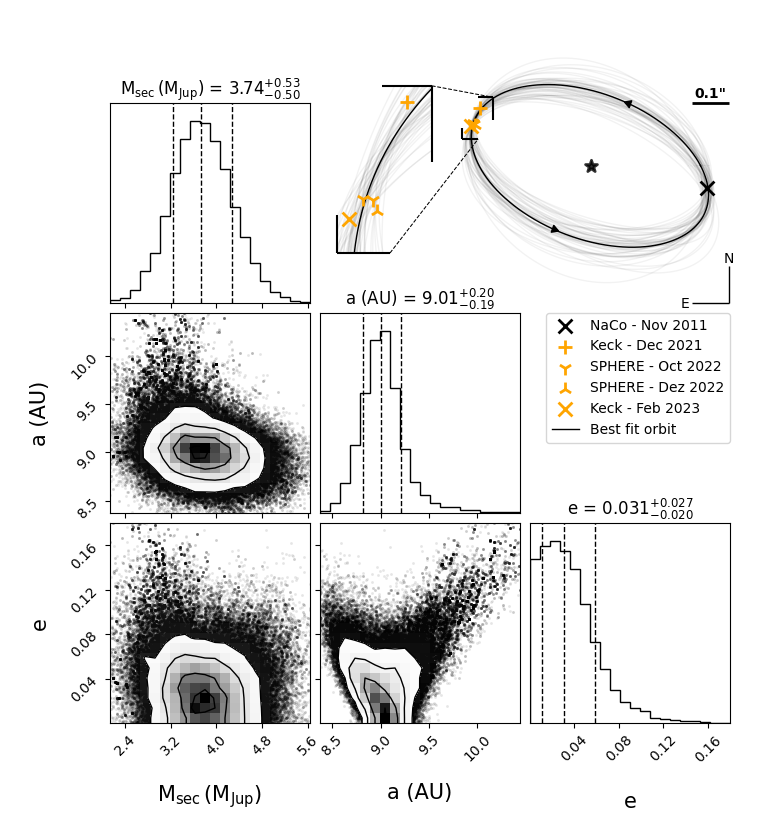
Figure 11: AF Lep b - parameters#
1. Imports#
[1]:
from copy import deepcopy
from pathlib import Path
import sys
import subprocess

import numpy as np
from astropy.io import fits
import matplotlib.pyplot as plt
from matplotlib import rcParams
from scipy.ndimage import gaussian_filter
from configparser import ConfigParser
import cmocean

from orvara import corner_modified
from orvara.orbit_plots import Orbit
from orvara.main_plotting import initialize_plot_options

from fours.utils.data_handling import read_fours_root_dir
2. Preparations#
This plot needs orvara to run the MCMC analysis and to create the plot. Make sure to install it.
Note: orvara and some packages used by orvara are not maintained. This leads to compatibility issues with numpy. We noticed that most issues can be solved by installing an over version of numpy. You can change your version by running:
[ ]:
%pip install numpy==1.23.0
This old numpy version may cause problems with other parts of the fours code. Be sure to revert the installation after the experiment is complete.
Information about the data#
The HIP number of AF Lep is 25486
The HGCA file can directly be copied from the orvara main directory. Filename: HGCA_vEDR3.fits
The RV data is taken from HIRES between 2002 and 2013 [Butler, R. P., Vogt, S. S., Laughlin, G., et al. 2017, AJ, 153, 208] and copied to the file AF_Lep_RV.txt
For the relative astrometry, apart from the NaCo L’-band data point the following other observations are available:
VLT/NACO 2011-Nov Bonse
Keck/NIRC2 2021-Dez Franson
VLT/SPHERE 2022-Oct Mesa
VLT/SPHERE 2022-Oct de Rosa
VLT/SPHERE 2022-Dez Mesa
Keck/NIRC2 2023-Feb Franson
The GAIA epochs and scan angles (GAIADataDir) are retrieved via: https://gaia.esac.esa.int/gost/
The original Hipparcos reduction for HIP1DataDir is retrieved from the following website: https://hipparcos-tools.cosmos.esa.int/cgi-bin/HIPcatalogueSearch.pl?hipiId=25486 Note, that the ID number at the end of the URL is the HIP number of the target in question.
For the HIP2DataDir, the reduction from van Leeuwen are downloaded from https://www.cosmos.esa.int/web/hipparcos/hipparcos-2 (under point 3)
Priors: As done in Branson et al. 2023, we set the host star mass prior to 1.2+-0.06 solar masses
MCMC setup: - 20 temperatures - 100 walkers - 5000 steps per walker
3. Create config for orvara#
Orvara needs a config file to run the MCMC analysis for the orbit fit.
We read in a general config file and adapt the links to match with the FOURS_ROOT_DIR.
[2]:
root_dir = Path(read_fours_root_dir())
Data in the FOURS_ROOT_DIR found. Location: /fast/mbonse/s4
Read the general config file.
[3]:
config = ConfigParser()
_= config.read(str(root_dir / Path("30_data/af_lep_parameters/config_all.ini")))
Set the directories and files needed.
[4]:
config['data_paths']['HGCAFile'] = str(root_dir / Path(config['data_paths']['HGCAFile']))
config['data_paths']['RVFile'] = str(root_dir / Path(config['data_paths']['RVFile']))
config['data_paths']['AstrometryFile'] = str(root_dir / Path(config['data_paths']['AstrometryFile']))
config['data_paths']['GaiaDataDir'] = str(root_dir / Path(config['data_paths']['GaiaDataDir']))
config['data_paths']['Hip1DataDir'] = str(root_dir / Path(config['data_paths']['Hip1DataDir']))
config['data_paths']['Hip2DataDir'] = str(root_dir / Path(config['data_paths']['Hip2DataDir']))

# if you want to use your own MCMC run change the McmcDataFile to the file created in the next step
config['plotting']['McmcDataFile'] = str(root_dir / Path(config['plotting']['McmcDataFile']))
[5]:
# Save the modified config file
config_path = root_dir / "30_data/af_lep_parameters/config_local.ini"
with open(config_path, 'w') as configfile:
    config.write(configfile)
4. Run orvara#
[6]:
# Define the output directory as a variable
output_dir = str(root_dir / "70_results/x4_af_lep/")

# Define the path to the config file
config_file = str(root_dir / "30_data/af_lep_parameters/config_local.ini")

# Construct the command using the variables
command = f"fit_orbit --output-dir {output_dir} {config_file}"

# Execute the command
result = subprocess.run(command, shell=True, capture_output=True, text=True)

# Print the output and any errors
print("Output:", result.stdout)
print("Error:", result.stderr)
Output: Unable to load relative RV data from file
Loadied 19 RV data points from file /fast/mbonse/s4/30_data/af_lep_parameters/AF_Lep_RV.txt
Loaded data from 1 RV instruments.
Loading astrometric data for 1 planets
Loaded 6 relative astrometric data points from file /fast/mbonse/s4/30_data/af_lep_parameters/AF_Lep_RelAstro_all.txt
Loading absolute astrometry data for Hip 25486
Recognized a 5-parameter fit in Gaia for Hip 25486
Not using companion proper motion from Gaia.
Using ptemcee.
Running MCMC ...
[                              ]  0%
[                              ]  1%
[                              ]  2%
[                              ]  3%
[#                             ]  4%
[#                             ]  5%
[#                             ]  6%
[##                            ]  7%
[##                            ]  8%
[##                            ]  9%
[###                           ] 10%
[###                           ] 11%
[###                           ] 12%
[####                          ] 13%
[####                          ] 14%
[####                          ] 15%
[####                          ] 16%
[#####                         ] 17%
[#####                         ] 18%
[#####                         ] 19%
[######                        ] 20%
[######                        ] 21%
[######                        ] 22%
[#######                       ] 23%
[#######                       ] 24%
[#######                       ] 25%
[########                      ] 26%
[########                      ] 27%
[########                      ] 28%
[########                      ] 29%
[#########                     ] 30%
[#########                     ] 31%
[#########                     ] 32%
[##########                    ] 33%
[##########                    ] 34%
[##########                    ] 35%
[###########                   ] 36%
[###########                   ] 37%
[###########                   ] 38%
[############                  ] 39%
[############                  ] 40%
[############                  ] 41%
[#############                 ] 42%
[#############                 ] 43%
[#############                 ] 44%
[#############                 ] 45%
[##############                ] 46%
[##############                ] 47%
[##############                ] 48%
[###############               ] 49%
[###############               ] 50%
[###############               ] 51%
[################              ] 52%
[################              ] 53%
[################              ] 54%
[#################             ] 55%
[#################             ] 56%
[#################             ] 57%
[#################             ] 58%
[##################            ] 59%
[##################            ] 60%
[##################            ] 61%
[###################           ] 62%
[###################           ] 63%
[###################           ] 64%
[####################          ] 65%
[####################          ] 66%
[####################          ] 67%
[#####################         ] 68%
[#####################         ] 69%
[#####################         ] 70%
[######################        ] 71%
[######################        ] 72%
[######################        ] 73%
[######################        ] 74%
[#######################       ] 75%
[#######################       ] 76%
[#######################       ] 77%
[########################      ] 78%
[########################      ] 79%
[########################      ] 80%
[#########################     ] 81%
[#########################     ] 82%
[#########################     ] 83%
[##########################    ] 84%
[##########################    ] 85%
[##########################    ] 86%
[##########################    ] 87%
[###########################   ] 88%
[###########################   ] 89%
[###########################   ] 90%
[############################  ] 91%
[############################  ] 92%
[############################  ] 93%
[############################# ] 94%
[############################# ] 95%
[############################# ] 96%
[##############################] 97%
[##############################] 98%
[##############################] 99%
[###############################]100%
Total Time: 276 seconds
Mean acceptance fraction (cold chain): 0.313616
Writing output to /fast/mbonse/s4/70_results/x4_af_lep/AF Lep b_chain001.fits

Error: [<astropy.io.fits.hdu.image.PrimaryHDU object at 0x152c716a8df0>, <astropy.io.fits.hdu.table.BinTableHDU object at 0x152c716293c0>]
This might take some time… Once completed there will be a new file in the 70_results/x4_af_lep folder which contains the results of your MCMC analysis. You can change config['plotting']['McmcDataFile'] to the file AF Lep b_chain000.fits or continue with our result af_lep_chain_all.fits.
5. Load the results of the MCMC analysis#
The orvara code is usually run from the command line. To generate the output in a jupyter notebook we have to set the command line arguments.
[7]:
original_argv = sys.argv.copy()
[8]:
sys.argv = ['script_name', config_file,
            '--output-dir', output_dir]
[9]:
# initialize the OP class object
OPs = initialize_plot_options(config)

# create the orbit object
orbit = Orbit(OPs)
Generating plots for target AF Lep b
[10]:
sys.argv = original_argv
6. Create the plot#
[11]:
def transform_to_sky(orbit, keepout_angle=259.2+90, dkoa=50):
    """
    Transform the orbit coordinates to sky coordinates.
    """

    # order the orbit coordinates
    ang_coords = np.array((deepcopy(orbit.relsep), ((deepcopy(orbit.PA+90)) * np.pi/180) % (2*np.pi))).T
    ang_coords = ang_coords[ang_coords[:, 1].argsort()]

    # convert to sky coordinates
    coords = np.array((ang_coords[:, 0] * np.cos(ang_coords[:, 1]), ang_coords[:, 0] * np.sin(ang_coords[:, 1])))

    return coords
[12]:
def get_xy_position(angle, distance_arsec):
    angle_radians = np.deg2rad(angle-90)
    distance = distance_arsec

    # Calculate x and y coordinates
    x = distance * np.cos(angle_radians)
    y = distance * np.sin(angle_radians)

    return -x, -y
[13]:
# sky coordinates for the most likely orbit
coords = transform_to_sky(orbit)
[14]:
# sky coordinates for the randomly selected orbits
sel_coords = []
for i in range(len(OPs.rand_idx)):
    orb = Orbit(OPs, step=OPs.rand_idx[i])
    sel_coords.append(transform_to_sky(orb))
[15]:
def plot_orbits(ax):
    for i in range(len(sel_coords)):
        ax.plot(sel_coords[i][0], sel_coords[i][1], color='k', alpha=0.05)

    ax.scatter(0, 0, marker="*", color="k", alpha=0.8, lw=2,zorder=2, s=80)

    msize = 100

    color_new = 'orange'

    datapoints = [['NaCo - Nov 2011', 259.2, 0.318, 'x', 'k'],
                  ['Keck - Dec 2021', 62.8, 0.338, '+', color_new],
                  ['SPHERE - Oct 2022', 70.2, 0.335, '1', color_new],
                  [None, 70.3, 0.339, '1', color_new],
                  ['SPHERE - Dez 2022', 70.8, 0.332, '2', color_new],
                  ['Keck - Feb 2023', 72.0, 0.342, 'x', color_new]]

    for d in datapoints:
        ax.scatter(*get_xy_position(d[1], d[2]),
                      marker=d[3],
                      color=d[4],
                      alpha=1, lw=2,
                      label=d[0],
                    zorder=2,
                      s=msize)

    ax.plot(coords[0], coords[1], color='k', label='Best fit orbit', zorder=1)

    ax.scatter(-0.1, -0.172, marker=(3, 0, 250), color='k')
    ax.scatter(0.1, 0.168, marker=(3, 0, 70), color='k')
[16]:
rcParams["lines.linewidth"] = 1.0
rcParams["axes.labelpad"] = 20.0
rcParams["xtick.labelsize"] = 10.0
rcParams["ytick.labelsize"] = 10.0

chain = OPs.chain

Mpri = chain['mpri']
npl = '%d' % (OPs.iplanet)
if OPs.cmref == 'msec_solar':
    Msec = chain['msec' + npl]         # in M_{\odot}
    labels=[r'$\mathrm{M_{pri}\, (M_{\odot})}$',
            r'$\mathrm{M_{sec}\, (M_{\odot})}$',
            'a (AU)',
            r'e',
            r'$\mathrm{i\, (^{\circ})}$']
else:
    Msec = chain['msec' + npl]*1989/1.898
    labels=[r'$\mathrm{M_{sec}\, (M_{Jup})}$', 'a (AU)', r'e']
Semimajor = chain['sau' + npl]
Ecc = chain['esino' + npl]**2 + chain['ecoso' + npl]**2
Inc = chain['inc' + npl]

chain = np.vstack([Msec, Semimajor, Ecc]).T

# in corner_modified, the error is modified to keep 2 significant figures
figure = corner_modified.corner(
    chain,
    labels=labels,
    quantiles=[0.16, 0.5, 0.84],
    range=[0.999 for l in labels],
    verbose=False,
    show_titles=True,
    title_kwargs={"fontsize": 12},
    hist_kwargs={"lw":1.},
    label_kwargs={"fontsize":15},
    xlabcord=(0.5,-0.45),
    ylabcord=(-0.45,0.5))

ax = plt.axes((0.56, 0.66, 0.41, 0.41))

plot_orbits(ax)

plt_lim = 0.42
ax.set_xlim(-plt_lim, plt_lim)
ax.set_ylim(-plt_lim, plt_lim)

size_position = -0.37
ax.hlines([-size_position-0.2, ],
             xmin=-size_position,
             xmax=-size_position - 0.1,
             color='k', lw=2)
ax.text(
    x=-size_position - 0.05 ,
    y=-size_position -0.195,
    s='0.1"', color='k', ha='center', va='bottom',
    fontsize=10,
    fontweight="bold")

ax.vlines(
    x=-size_position,
    ymin=size_position,
    ymax=size_position+0.1,
    color='k')

ax.hlines(
    y=size_position,
    xmin=-size_position-0.1,
    xmax=-size_position,
    color='k')

ax.text(
    x=-size_position,
    y=size_position+0.1,
    s='N',
    color='k',
    ha='center',
    va='bottom',
    fontsize=10)

ax.text(
    x=-size_position-0.105,
    y=size_position-0.003,
    s='E',
    color='k',
    ha='right',
    va='center',
    fontsize=10)

ax.set_xticks([])
ax.set_yticks([])

ax.patch.set_alpha(0.0001)
ax.spines[['right', 'top', 'left', 'bottom']].set_visible(False)

ax.legend(loc='upper center',
          bbox_to_anchor=(0.65, 0.05),
          ncol=1, fontsize=10)


midpoint = np.array(get_xy_position(70.2, 0.335)) + np.array((0.005, 0.013))
delta = np.array((0.02, 0.035))

ax2 = plt.axes((0.43, 0.75, 0.22*delta[0]/delta[1], 0.22))
plot_orbits(ax2)

#ax2.patch.set_alpha(0.0001)
ax2.spines[['right', 'top', 'left', 'bottom']].set_visible(False)
ax2.set_xticks([])
ax2.set_yticks([])


ax2.set_xlim(midpoint[0]-delta[0], midpoint[0]+delta[0])
ax2.set_ylim(midpoint[1]-delta[1], midpoint[1]+delta[1])

ax3 = plt.axes((0, 0, 1, 1), frameon=False)
ax3.set_xticks([])
ax3.set_yticks([])

lw = 1.5
bracket_i = {'x': 0.555,
             'y': 0.97,
             'dy': 0.1,
             'scale': 0.65}

bracket_o = {'x': 0.635,
             'y': 0.955,
             'dy': 0.03,
             'scale': 0.65}

stop_i = {'x': 0.43,
             'y': 0.75,
             'dy': 0.05,
             'scale': 1.4}

stop_o = {'x': 0.595,
             'y': 0.9,
             'dy': 0.015,
             'scale': 1.4}


ax3.vlines(x=bracket_i['x'],
           ymin=bracket_i['y']-bracket_i['dy'],
           ymax=bracket_i['y'],
           color='k', lw=lw)
ax3.hlines(y=bracket_i['y'],
           xmin=bracket_i['x'] - bracket_i['dy'] * bracket_i['scale'],
           xmax=bracket_i['x'],
           color='k', lw=lw)

ax3.vlines(x=bracket_o['x'],
           ymin=bracket_o['y']-bracket_o['dy'],
           ymax=bracket_o['y'],
           color='k', lw=lw)
ax3.hlines(y=bracket_o['y'],
           xmin=bracket_o['x'] - bracket_o['dy'] * bracket_o['scale'],
           xmax=bracket_o['x'],
           color='k', lw=lw)

ax3.vlines(x=stop_i['x'],
           ymin=stop_i['y'],
           ymax=stop_i['y'] + stop_i['dy'],
           color='k', lw=lw)
ax3.hlines(y=stop_i['y'],
           xmin=stop_i['x'],
           xmax=stop_i['x'] + stop_i['dy'] * stop_i['scale'],
           color='k', lw=lw)

ax3.vlines(x=stop_o['x'],
           ymin=stop_o['y'],
           ymax=stop_o['y'] + stop_o['dy'],
           color='k', lw=lw)
ax3.hlines(y=stop_o['y'],
           xmin=stop_o['x'],
           xmax=stop_o['x'] + stop_o['dy'] * stop_o['scale'],
           color='k', lw=lw)

ax3.plot([bracket_i['x'], bracket_o['x']], [bracket_i['y'], bracket_o['y']], color='k', lw=lw/2, ls='--')
ax3.plot([stop_i['x'] + stop_i['dy'] * stop_i['scale'],
          stop_o['x'] + stop_o['dy'] * stop_o['scale']],
         [stop_i['y'], stop_o['y']], color='k', lw=lw/2, ls='--')

ax3.set_xlim(0, 1)
ax3.set_ylim(0, 1)

# save the figure
plt.savefig("./final_plots/06_af_lep_orbit.pdf", bbox_inches='tight')