MCMC for AF Lep b#
1. Imports#
[1]:
import os
os.environ['OMP_NUM_THREADS'] = '5'
[ ]:
from pathlib import Path
from tqdm import tqdm

import numpy as np

# Plotting
import cmocean
import matplotlib.pylab as plt
color_map = cmocean.cm.ice
import seaborn as sns
from matplotlib.lines import Line2D

# Methods
import pynpoint as pp
from pynpoint.core.dataio import OutputPort, InputPort
from pynpoint.readwrite.hdf5reading import Hdf5ReadingModule

from fours.utils.pca import pca_psf_subtraction_gpu
from fours.utils.data_handling import read_fours_root_dir

# Evaluation
from applefy.detections.uncertainty import compute_detection_uncertainty
from applefy.utils.photometry import AperturePhotometryMode
from applefy.statistics import TTest
2. All directories needed#
[ ]:
root_dir = Path(read_fours_root_dir())
[4]:
experiment_root_dir = root_dir / Path("70_results/x2_af_lep/MCMC/")
[5]:
fwhm = 3.6
3. Estimate the Photometry and astrometry with PynPoint#
3.1 Create the PynPoint database#
[6]:
pipeline = pp.Pypeline(
    working_place_in=str(experiment_root_dir),
    input_place_in=str(experiment_root_dir),
    output_place_in=str(experiment_root_dir))
================
PynPoint v0.10.1
================

A new version (0.11.0) is available!

Want to stay informed about updates, bug fixes, and new features?
Please consider using the 'Watch' button on the Github page:
https://github.com/PynPoint/PynPoint

Working place: /home/ipa/quanz/user_accounts/mbonse/2023_S4/70_results/x2_af_lep/MCMC
Input place: /home/ipa/quanz/user_accounts/mbonse/2023_S4/70_results/x2_af_lep/MCMC
Output place: /home/ipa/quanz/user_accounts/mbonse/2023_S4/70_results/x2_af_lep/MCMC

Database: /home/ipa/quanz/user_accounts/mbonse/2023_S4/70_results/x2_af_lep/MCMC/PynPoint_database.hdf5
Configuration: /home/ipa/quanz/user_accounts/mbonse/2023_S4/70_results/x2_af_lep/MCMC/PynPoint_config.ini

Number of CPUs: 32
Number of threads: 5
3.2 Read in the HDF5 file#
[7]:
read_data_module = Hdf5ReadingModule(
    name_in="01_read_data",
    input_filename="HD35850_294_088_C-0085_A_.hdf5",
    input_dir=str(root_dir / Path("30_data")),
    tag_dictionary={"object_selected" : "object_selected",
                    "psf_selected" : "psf_selected"})
[8]:
pipeline.add_module(read_data_module)
[9]:
pipeline.run_module("01_read_data")
-----------------
Hdf5ReadingModule
-----------------

Module name: 01_read_data
Reading HDF5 file... [DONE]
Output ports: object_selected (13809, 165, 165), psf_selected (1526, 23, 23)
3.3 Cut and stack the science data for faster PCA iterations#
[10]:
science_data = pipeline.get_data("object_selected")
angles = pipeline.get_attribute("object_selected", "PARANG", static=False)

print(science_data.shape)
(13809, 165, 165)
(13809,)
[11]:
science_data_cut = science_data[:, 25:-25, 25:-25]
[12]:
binning = 5  # stack every 5 frames
angles_stacked = np.array([
    np.mean(i)
    for i in np.array_split(angles, int(len(angles) / binning))])
science_stacked = np.array([
    np.mean(i, axis=0)
    for i in np.array_split(science_data_cut, int(len(angles) / binning))])
[13]:
obj_port = OutputPort(
    "01_science_prep",
    pipeline.m_data_storage)
obj_port.set_all(science_stacked)
[14]:
input_port = InputPort(
    "object_selected",
    pipeline.m_data_storage)
obj_port.copy_attributes(input_port)
[15]:
pipeline.set_attribute("01_science_prep", "PARANG", angles_stacked, False)
3.4 Find the best number of PCA components#
[16]:
science_data_prep = pipeline.get_data("01_science_prep")
angles_prep = pipeline.get_attribute("01_science_prep", "PARANG", static=False)
angles_prep = np.deg2rad(angles_prep)
[17]:
print(science_data_prep.shape)
print(angles_prep.shape)
(2761, 115, 115)
(2761,)
[18]:
num_components = np.arange(5, 200, 10)
[19]:
pca_residuals = pca_psf_subtraction_gpu(
    images=science_data_prep,
    angles=angles_prep,
    pca_numbers=num_components,
    device="cpu",
    approx_svd=2000,
    verbose = True)
Compute PCA basis ...[DONE]
Compute PCA residuals ...
100%|███████████████████████████████████████████████████████████████████████████████████████████████████████████████████████████████████████████████████████████████████████| 20/20 [00:10<00:00, 1.83it/s]
[DONE]
[20]:
init_planet_position  = np.array((68.55, 54.78)) # Result from previous mcmc
# Use pixel values spaced by the FWHM
photometry_mode_planet = AperturePhotometryMode("AS", search_area=0.5, psf_fwhm_radius=fwhm/2)
photometry_mode_noise = AperturePhotometryMode("AS", psf_fwhm_radius=fwhm/2)
[21]:
all_snr_pca = []
for i in tqdm(range(len(num_components))):
    _, _, snr_mean = compute_detection_uncertainty(
        frame=pca_residuals[i],
        planet_position=init_planet_position,
        statistical_test=TTest(),
        psf_fwhm_radius=fwhm,
        photometry_mode_planet=photometry_mode_planet,
        photometry_mode_noise=photometry_mode_noise,
        safety_margin=1.,
        num_rot_iter=50)

    all_snr_pca.append(np.round(np.mean(snr_mean), 1))
100%|███████████████████████████████████████████████████████████████████████████████████████████████████████████████████████████████████████████████████████████████████████| 20/20 [00:06<00:00, 2.89it/s]
[22]:
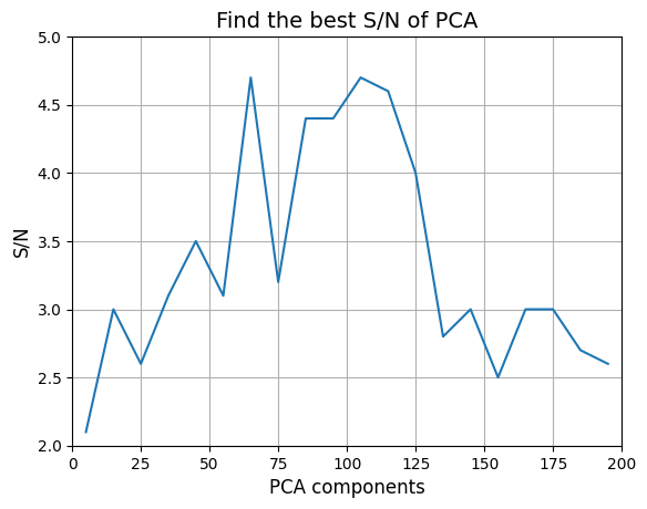
plt.plot(num_components, all_snr_pca)
plt.ylabel("S/N", fontsize=12)
plt.xlabel("PCA components", fontsize=12)
plt.title("Find the best S/N of PCA", fontsize=14)

plt.xlim(0, 200)
plt.ylim(2, 5)
plt.grid()
[23]:
best_num_pca = num_components[np.argmax(all_snr_pca)]
print("The best number of components is: " + str(best_num_pca))
print("The peak S/N is : " + str(np.max(all_snr_pca)))
The best number of components is: 65
The peak S/N is : 4.7
[24]:
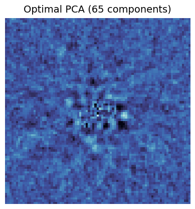
pca_residual_frame = pca_residuals[np.argmax(all_snr_pca)]
median= np.median(pca_residual_frame)
scale = np.max(np.abs(pca_residual_frame))
zoom = 15

plt.imshow(
    pca_residual_frame[zoom:-zoom, zoom:-zoom],
    cmap=color_map,
    vmin=median - scale*0.5, vmax=median + scale*0.8,
    origin="lower")
plt.axis("off")
plt.title("Optimal PCA (65 components)", fontsize=14,y=1.01)
[24]:
Text(0.5, 1.01, 'Optimal PCA (65 components)')
3.5 Create a Master Template for the PSF#
[25]:
psf_frames = pipeline.get_data("psf_selected")
[26]:
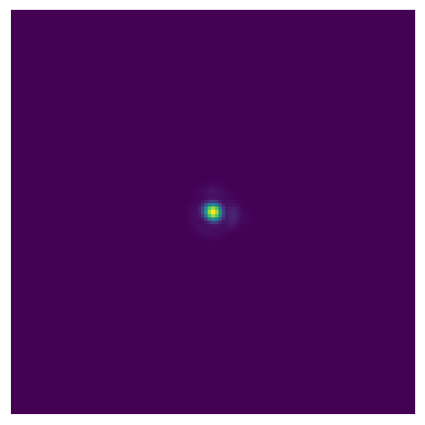
psf_template = np.median(psf_frames, axis=0)
[27]:
# pad the psf template
padded_psf = np.pad(psf_template,
                  pad_width=((46, 46), (46, 46)),
                  mode='constant',
                  constant_values=0)

plt.imshow(padded_psf)
plt.axis("off")
[27]:
(-0.5, 114.5, 114.5, -0.5)
[28]:
psf_port = OutputPort("01_psf_padded",
                      pipeline.m_data_storage)
psf_port.set_all(np.expand_dims(padded_psf, axis=0))
3.6 Simplex minimization, used as initialization for MCMC#
[29]:
simplex_module = pp.SimplexMinimizationModule(
    name_in='03_simplex',
    image_in_tag='01_science_prep',
    psf_in_tag='01_psf_padded',
    res_out_tag='03_simplex_residual',
    flux_position_tag='03_simplex_result',
    position=(init_planet_position[0], init_planet_position[1]),
    magnitude=9.5,
    psf_scaling=-1/0.0179,  # The data is taken with an ND filter
    merit='hessian',
    tolerance=0.1,
    pca_number=int(best_num_pca),
    residuals='mean',
    offset=2)
[30]:
pipeline.add_module(simplex_module)
pipeline.run_module('03_simplex')
-------------------------
SimplexMinimizationModule
-------------------------

Module name: 03_simplex
Input ports: 01_science_prep (2761, 115, 115), 01_psf_padded (1, 115, 115)
Input parameters:
   - Number of principal components = [65]
   - Figure of merit = hessian
   - Residuals type = mean
   - Absolute tolerance (pixels/mag) = 0.1
   - Maximum offset = 2
   - Guessed position (x, y) = (68.55, 54.78)
   - Aperture position (x, y) = (69, 55)
   - Aperture radius (pixels) = 3
Image center (y, x) = (57.0, 57.0)
Simplex minimization... 65 PC - chi^2 = 1.52e+01 [DONE]
Best-fit parameters:
   - Position (x, y) = (68.78, 54.75)
   - Separation (mas) = 323.70
   - Position angle (deg) = 259.19
   - Contrast (mag) = 9.98
Output ports: 03_simplex_residual (41, 115, 115), 03_simplex_result (41, 6)
[31]:
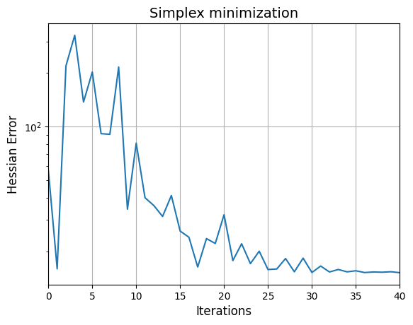
simplex_results = pipeline.get_data('03_simplex_result')
[32]:
# Simplex Error
plt.plot(simplex_results[:, -1])
plt.yscale("log")
plt.xlabel("Iterations", fontsize=12)
plt.ylabel("Hessian Error", fontsize=12)
plt.title("Simplex minimization", fontsize=14)
plt.xlim(0, 40)
plt.grid()
[33]:
best_idx = np.argmin(simplex_results[:, -1])
best_idx
[33]:
40
[34]:
simplex_best_result = simplex_results[best_idx, :]
simplex_best_result
[34]:
array([ 68.77608758,  54.75116433,   0.32370005, 259.18860748,
         9.98117147,  15.16769487])
[35]:
residual_no_planet = pipeline.get_data('03_simplex_residual')[best_idx]
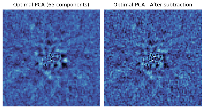
[36]:
fig, (ax1, ax2) = plt.subplots(1, 2, figsize=(8, 5))

# Plot the original residual
median= np.median(pca_residual_frame)
scale = np.max(np.abs(pca_residual_frame))
zoom = 15

ax1.imshow(
    pca_residual_frame[zoom:-zoom, zoom:-zoom],
    cmap=color_map,
    vmin=median - scale*0.5, vmax=median + scale*0.8,
    origin="lower")

ax1.axis("off")
ax1.set_title("Optimal PCA (65 components)", fontsize=14,y=1.01)

# Plot the residual without the planet
ax2.imshow(
    residual_no_planet[zoom:-zoom, zoom:-zoom],
    cmap=color_map,
    vmin=median - scale*0.5, vmax=median + scale*0.8,
    origin="lower")

ax2.axis("off")
ax2.set_title("Optimal PCA - After subtraction", fontsize=14,y=1.01)

plt.tight_layout()
3.7 Run MCMC to get an estimate of the Error#
[54]:
# Bounds for the MCMC
# Separations +- 100 mas
# Angle +- 10 deg
# Contrast +- 1 mag

dsep, dphi, dcontrast = 0.1, 10, 1.0

mcmc_module = pp.MCMCsamplingModule(
    name_in='04_MCMC_planet',
    image_in_tag='01_science_prep',
    psf_in_tag='01_psf_padded',
    chain_out_tag='04_MCMC_chain',
    param=tuple(simplex_best_result[2:5]),
    bounds=((simplex_best_result[2]-dsep, simplex_best_result[2]+dsep),
            (simplex_best_result[3]-dphi, simplex_best_result[3]+dphi),
            (simplex_best_result[4]-dcontrast, simplex_best_result[4]+dcontrast)),
    nwalkers=100,
    nsteps=500,
    psf_scaling=-1/0.0179, # ND filter
    pca_number=int(best_num_pca),
    mask=None,
    extra_rot=0.0,
    merit='hessian',
    residuals='mean',
    resume=True)
[ ]:
pipeline.add_module(mcmc_module)
pipeline.run_module('04_MCMC_planet')
3.8 Plot the result#
[56]:
mcmc_results = pipeline.get_data('04_MCMC_chain')
[85]:
mcmc_angles = mcmc_results[-50:,:, 1].flatten()
mcmc_separations = mcmc_results[-50:,:, 0].flatten() * 1000
mcmc_contrast = mcmc_results[-50:,:, 2].flatten()
The true north in NACO can be off by about 0.5 deg. Rameau et. al 2013 calibtrated north for our dataset. We use their calibration to update the position angles
[146]:
mcmc_angles = mcmc_angles - 0.38 # the error is negligible
[147]:
def get_statistic(sample_in):
    median = np.median(sample_in)
    low = np.quantile(sample_in, 0.16)
    high = np.quantile(sample_in, 0.84)

    plus = high - median
    minus = low - median

    return np.round(median, 2), np.round(plus, 2), np.round(minus, 2)
[148]:
print(get_statistic(mcmc_angles))
median_angle, plus_angle, minus_angle = get_statistic(mcmc_angles)
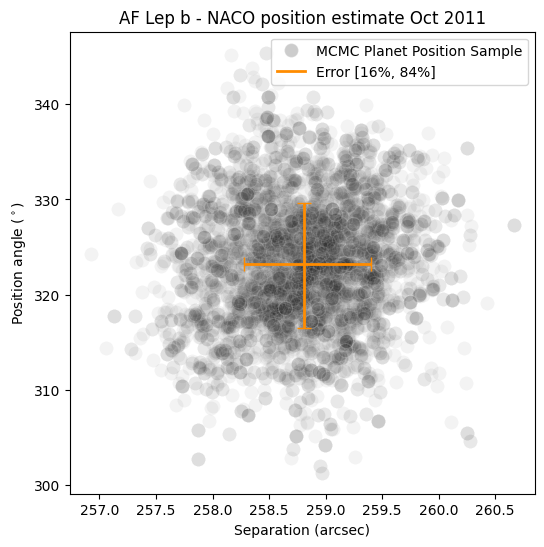
(258.81, 0.53, -0.59)
[149]:
print(get_statistic(mcmc_separations))
median_separations, plus_separations, minus_separations = get_statistic(mcmc_separations)
(323.24, 6.71, -6.44)
[163]:
x = mcmc_angles
y = mcmc_separations

# Draw a combo histogram and scatterplot with density contours
f, ax = plt.subplots(figsize=(6, 6))
sns.scatterplot(
    x=mcmc_angles,
    y=mcmc_separations,
    s=100,
    color=".15",
    alpha=0.05,
    label='MCMC planet position sample')

ax.errorbar(
    x=median_angle,
    xerr=np.array([plus_angle, -minus_angle]).reshape(2, 1),
    y=median_separations,
    yerr=np.array([plus_separations, -minus_separations]).reshape(2, 1),
    c='darkorange',
    lw=2,
    capsize=5)

legend_elements = [Line2D([0], [0], marker='o', color='w', label='MCMC Planet Position Sample',
                          markerfacecolor='k', markersize=10, alpha=0.2),
                   Line2D([0], [0], color='darkorange', lw=2, label='Error [16%, 84%]')]

ax.legend(handles=legend_elements, loc='best')

ax.ticklabel_format(useOffset=False)
ax.set_xlabel('Separation (arcsec)')
ax.set_ylabel(r'Position angle ($^\circ$)')
ax.set_title('AF Lep b - NACO position estimate Oct 2011')
f.savefig('final_plots/x1_AF_Lep_NACO_position_estimate.pdf', bbox_inches='tight')
plt.show()
[157]:
print(get_statistic(mcmc_contrast))
median_contrast, plus_contrast, minus_contrast = get_statistic(mcmc_contrast)
(10.03, 0.13, -0.12)
[155]:
host_mag = 4.93
host_error = 0.01
[160]:
apparent_mag = np.round(median_contrast + host_mag, 2)
apparent_mag
[160]:
14.96
[161]:
Abs_mag = 12.81